Homework8
Sam Troast
2025-03-19
Question 1
library(ggplot2) # for graphics
library(MASS) # for maximum likelihood estimation

# quick and dirty, a truncated normal distribution to work on the solution set

# read in data vector
z <- rnorm(n=3000,mean=0.2)
z <- data.frame(1:3000,z)
names(z) <- list("ID","myVar")
z <- z[z$myVar>0,]
str(z)
## 'data.frame': 1751 obs. of 2 variables:
## $ ID : int 1 3 4 5 7 8 9 11 12 13 ...
## $ myVar: num 0.558 1.255 0.677 0.502 1.04 ...summary(z$myVar)## Min. 1st Qu. Median Mean 3rd Qu. Max.
## 0.000334 0.364966 0.743118 0.866502 1.204638 3.490032# plot histogram of data
p1 <- ggplot(data=z, aes(x=myVar, y=..density..)) +
geom_histogram(color="grey60",fill="cornsilk", linewidth=0.2)
print(p1)## Warning: The dot-dot notation (`..density..`) was deprecated in ggplot2 3.4.0.
## ℹ Please use `after_stat(density)` instead.
## This warning is displayed once every 8 hours.
## Call `lifecycle::last_lifecycle_warnings()` to see where this warning was
## generated.## `stat_bin()` using `bins = 30`. Pick better value with `binwidth`.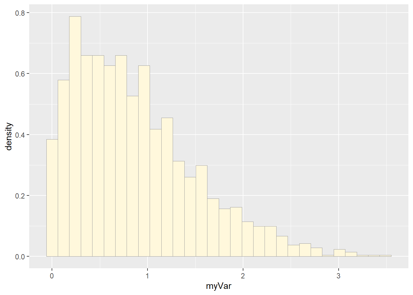
# add empirical density curve
p1 <-  p1 +  geom_density(linetype="dotted",size=0.75)
## Warning: Using `size` aesthetic for lines was deprecated in ggplot2 3.4.0.
## ℹ Please use `linewidth` instead.
## This warning is displayed once every 8 hours.
## Call `lifecycle::last_lifecycle_warnings()` to see where this warning was
## generated.print(p1)## `stat_bin()` using `bins = 30`. Pick better value with `binwidth`.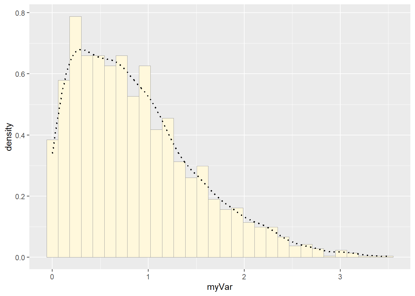
# get maximum likelihood parameters for normal
normPars <- fitdistr(z$myVar,"normal")
print(normPars)
## mean sd
## 0.86650190 0.63678077
## (0.01521762) (0.01076049)str(normPars)## List of 5
## $ estimate: Named num [1:2] 0.867 0.637
## ..- attr(*, "names")= chr [1:2] "mean" "sd"
## $ sd : Named num [1:2] 0.0152 0.0108
## ..- attr(*, "names")= chr [1:2] "mean" "sd"
## $ vcov : num [1:2, 1:2] 0.000232 0 0 0.000116
## ..- attr(*, "dimnames")=List of 2
## .. ..$ : chr [1:2] "mean" "sd"
## .. ..$ : chr [1:2] "mean" "sd"
## $ n : int 1751
## $ loglik : num -1694
## - attr(*, "class")= chr "fitdistr"normPars$estimate["mean"] # note structure of getting a named attribute## mean
## 0.8665019# plot normal probability density
meanML <- normPars$estimate["mean"]
sdML <- normPars$estimate["sd"]
xval <- seq(0,max(z$myVar),len=length(z$myVar))
stat <- stat_function(aes(x = xval, y = ..y..), fun = dnorm, colour="red", n = length(z$myVar), args = list(mean = meanML, sd = sdML))
p1 + stat## `stat_bin()` using `bins = 30`. Pick better value with `binwidth`.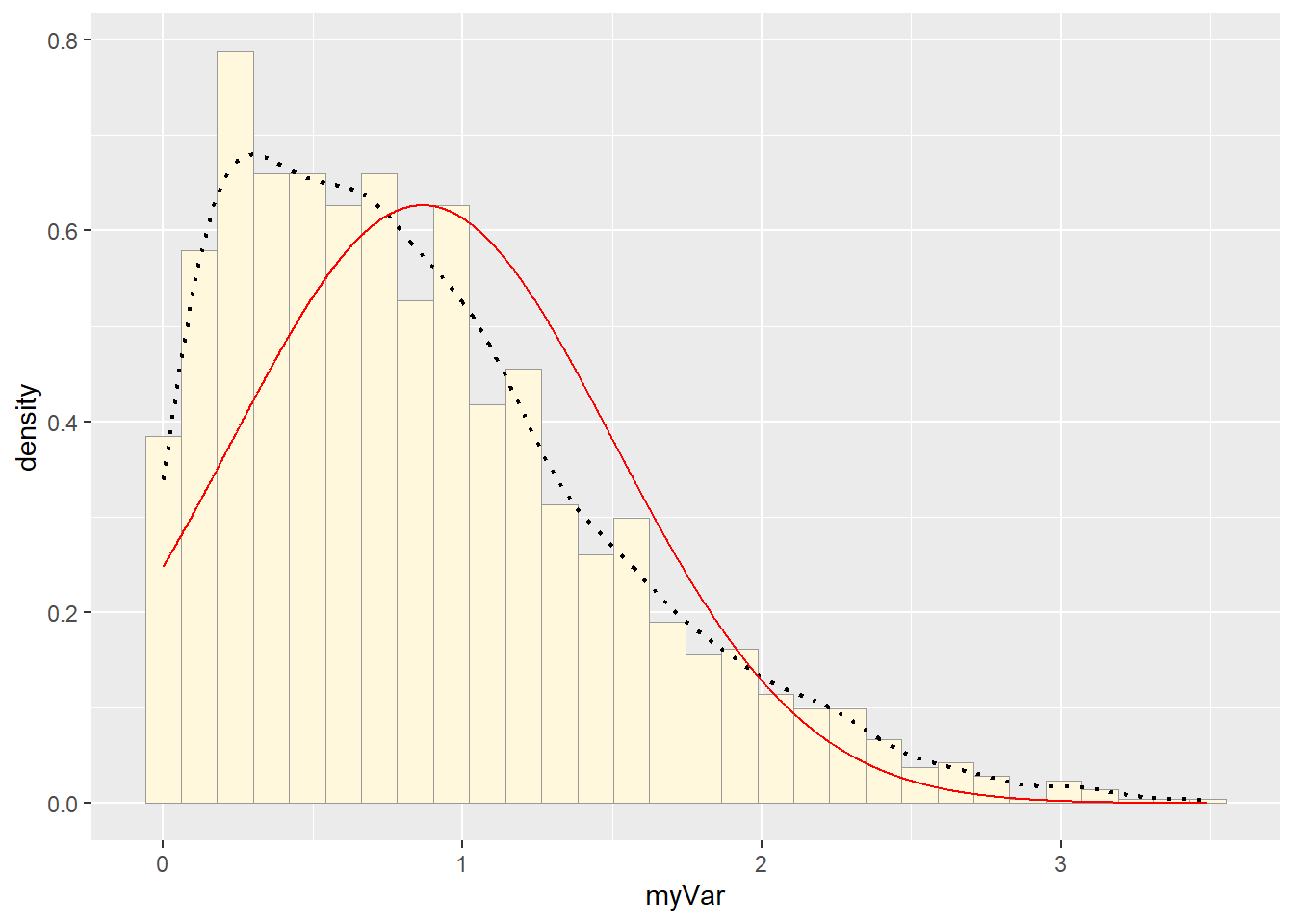
# plot exponential probability density
expoPars <- fitdistr(z$myVar,"exponential")
rateML <- expoPars$estimate["rate"]

stat2 <- stat_function(aes(x = xval, y = ..y..), fun = dexp, colour="blue", n = length(z$myVar), args = list(rate=rateML))
 p1 + stat + stat2
## `stat_bin()` using `bins = 30`. Pick better value with `binwidth`.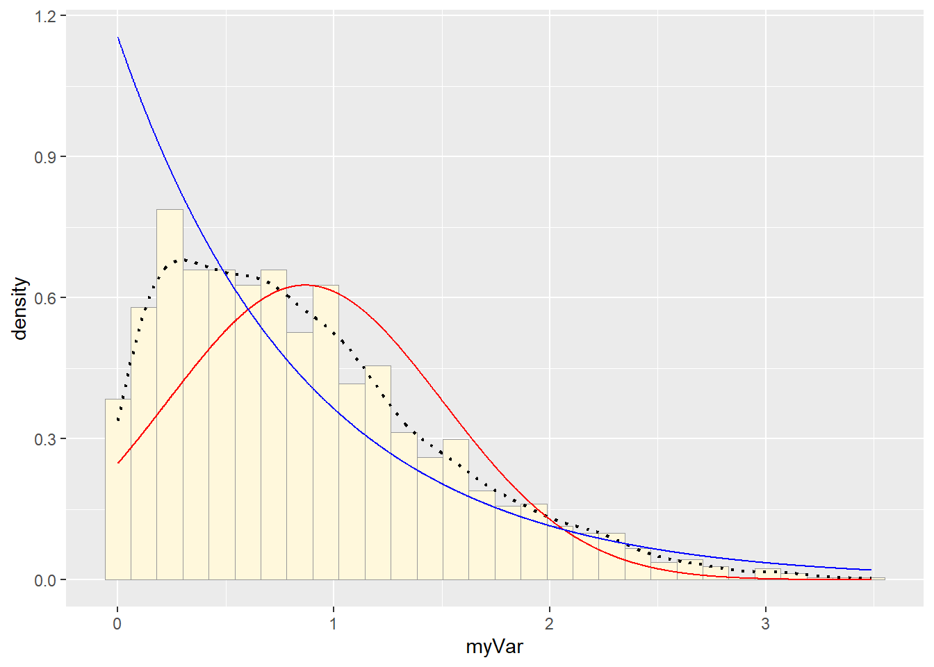
# plot uniform probability density
stat3 <- stat_function(aes(x = xval, y = ..y..), fun = dunif, colour="darkgreen", n = length(z$myVar), args = list(min=min(z$myVar), max=max(z$myVar)))
 p1 + stat + stat2 + stat3
## `stat_bin()` using `bins = 30`. Pick better value with `binwidth`.
# plot gamma probability density
gammaPars <- fitdistr(z$myVar,"gamma")
## Warning in densfun(x, parm[1], parm[2], ...): NaNs produced## Warning in densfun(x, parm[1], parm[2], ...): NaNs produced
## Warning in densfun(x, parm[1], parm[2], ...): NaNs produced
## Warning in densfun(x, parm[1], parm[2], ...): NaNs produced
## Warning in densfun(x, parm[1], parm[2], ...): NaNs produced
## Warning in densfun(x, parm[1], parm[2], ...): NaNs produced
## Warning in densfun(x, parm[1], parm[2], ...): NaNs producedshapeML <- gammaPars$estimate["shape"]
rateML <- gammaPars$estimate["rate"]
stat4 <- stat_function(aes(x = xval, y = ..y..), fun = dgamma, colour="brown", n = length(z$myVar), args = list(shape=shapeML, rate=rateML))
p1 + stat + stat2 + stat3 + stat4## `stat_bin()` using `bins = 30`. Pick better value with `binwidth`.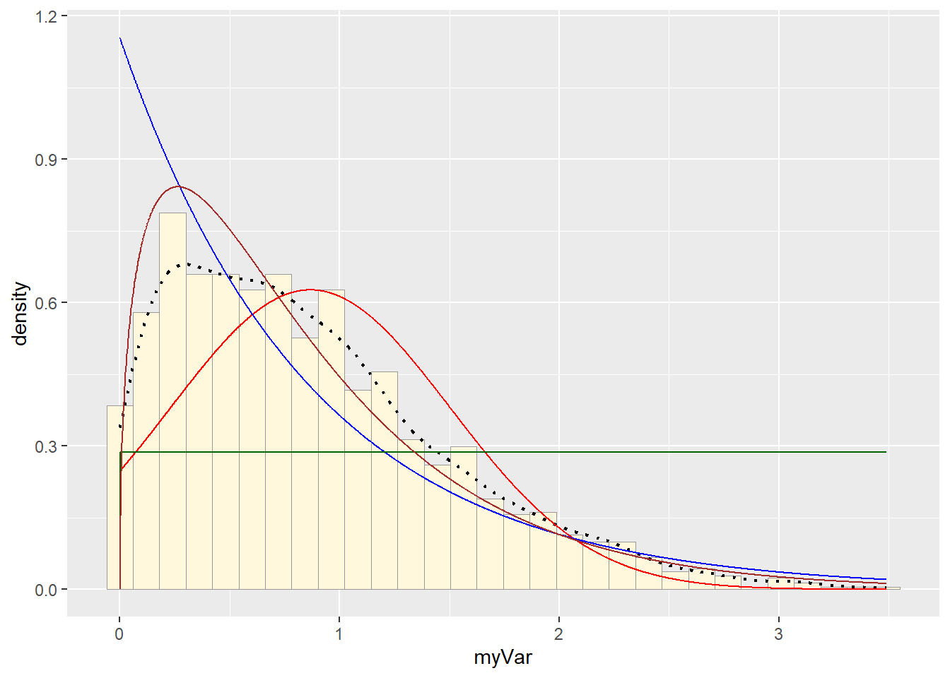
# plot beta probability density
pSpecial <- ggplot(data=z, aes(x=myVar/(max(myVar + 0.1)), y=..density..)) +
  geom_histogram(color="grey60",fill="cornsilk",size=0.2) +
  xlim(c(0,1)) +
  geom_density(size=0.75,linetype="dotted")

betaPars <- fitdistr(x=z$myVar/max(z$myVar + 0.1),start=list(shape1=1,shape2=2),"beta")
## Warning in densfun(x, parm[1], parm[2], ...): NaNs produced
## Warning in densfun(x, parm[1], parm[2], ...): NaNs produced
## Warning in densfun(x, parm[1], parm[2], ...): NaNs produced
## Warning in densfun(x, parm[1], parm[2], ...): NaNs producedshape1ML <- betaPars$estimate["shape1"]
shape2ML <- betaPars$estimate["shape2"]
statSpecial <- stat_function(aes(x = xval, y = ..y..), fun = dbeta, colour="orchid", n = length(z$myVar), args = list(shape1=shape1ML,shape2=shape2ML))
pSpecial + statSpecial## `stat_bin()` using `bins = 30`. Pick better value with `binwidth`.## Warning: Removed 2 rows containing missing values or values outside the scale range
## (`geom_bar()`).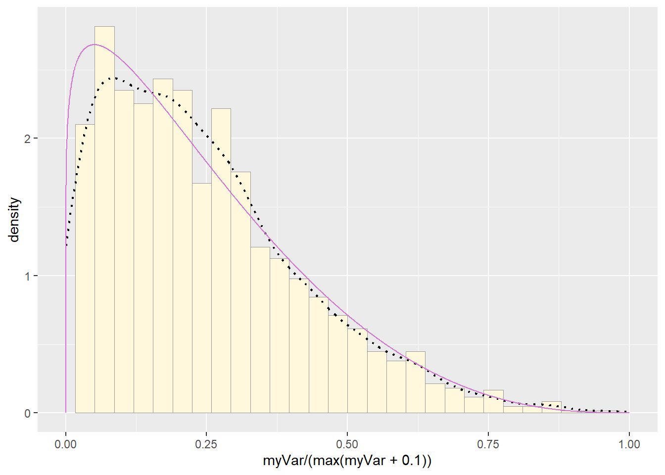
Question 2
library(tidyverse)## ── Attaching core tidyverse packages ──────────────────────── tidyverse 2.0.0 ──
## ✔ dplyr 1.1.4 ✔ readr 2.1.5
## ✔ forcats 1.0.0 ✔ stringr 1.5.1
## ✔ lubridate 1.9.4 ✔ tibble 3.2.1
## ✔ purrr 1.0.2 ✔ tidyr 1.3.1
## ── Conflicts ────────────────────────────────────────── tidyverse_conflicts() ──
## ✖ dplyr::filter() masks stats::filter()
## ✖ dplyr::lag() masks stats::lag()
## ✖ dplyr::select() masks MASS::select()
## ℹ Use the conflicted package (<http://conflicted.r-lib.org/>) to force all conflicts to become errorsz0 <- data.frame(starwars)
z <- na.omit(starwars)
view(z)
# plot histogram of data
p1 <- ggplot(data=z, aes(x=height, y=..density..)) +
geom_histogram(color="grey60",fill="cornsilk", linewidth=0.2)
print(p1)## `stat_bin()` using `bins = 30`. Pick better value with `binwidth`.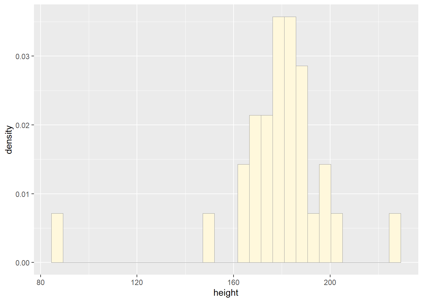
# add empirical density curve
p1 <- p1 + geom_density(linetype="dotted",size=0.75)
print(p1)## `stat_bin()` using `bins = 30`. Pick better value with `binwidth`.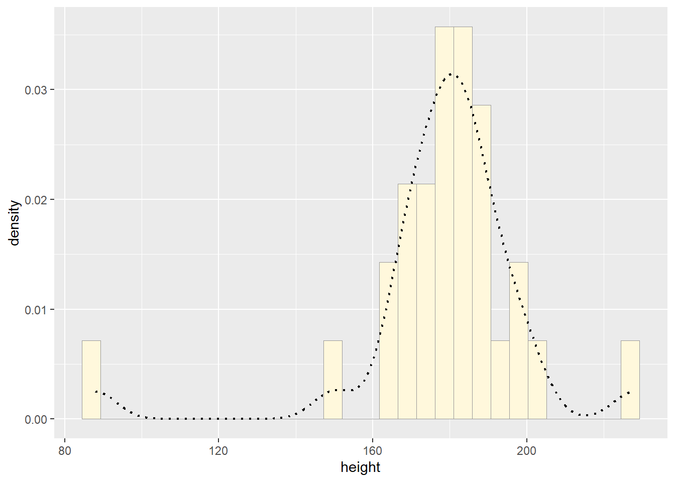
# get maximum likelihood parameters for normal
normPars <- fitdistr(z$height,"normal")
print(normPars)## mean sd
## 178.655172 22.009835
## ( 4.087124) ( 2.890033)str(normPars)## List of 5
## $ estimate: Named num [1:2] 179 22
## ..- attr(*, "names")= chr [1:2] "mean" "sd"
## $ sd : Named num [1:2] 4.09 2.89
## ..- attr(*, "names")= chr [1:2] "mean" "sd"
## $ vcov : num [1:2, 1:2] 16.7 0 0 8.35
## ..- attr(*, "dimnames")=List of 2
## .. ..$ : chr [1:2] "mean" "sd"
## .. ..$ : chr [1:2] "mean" "sd"
## $ n : int 29
## $ loglik : num -131
## - attr(*, "class")= chr "fitdistr"normPars$estimate["mean"] # note structure of getting a named attribute## mean
## 178.6552# plot normal probability density
meanML <- normPars$estimate["mean"]
sdML <- normPars$estimate["sd"]
xval <- seq(0,max(z$height),len=length(z$height))
stat <- stat_function(aes(x = xval, y = ..y..), fun = dnorm, colour="red", n = length(z$height), args = list(mean = meanML, sd = sdML))
p1 + stat## `stat_bin()` using `bins = 30`. Pick better value with `binwidth`.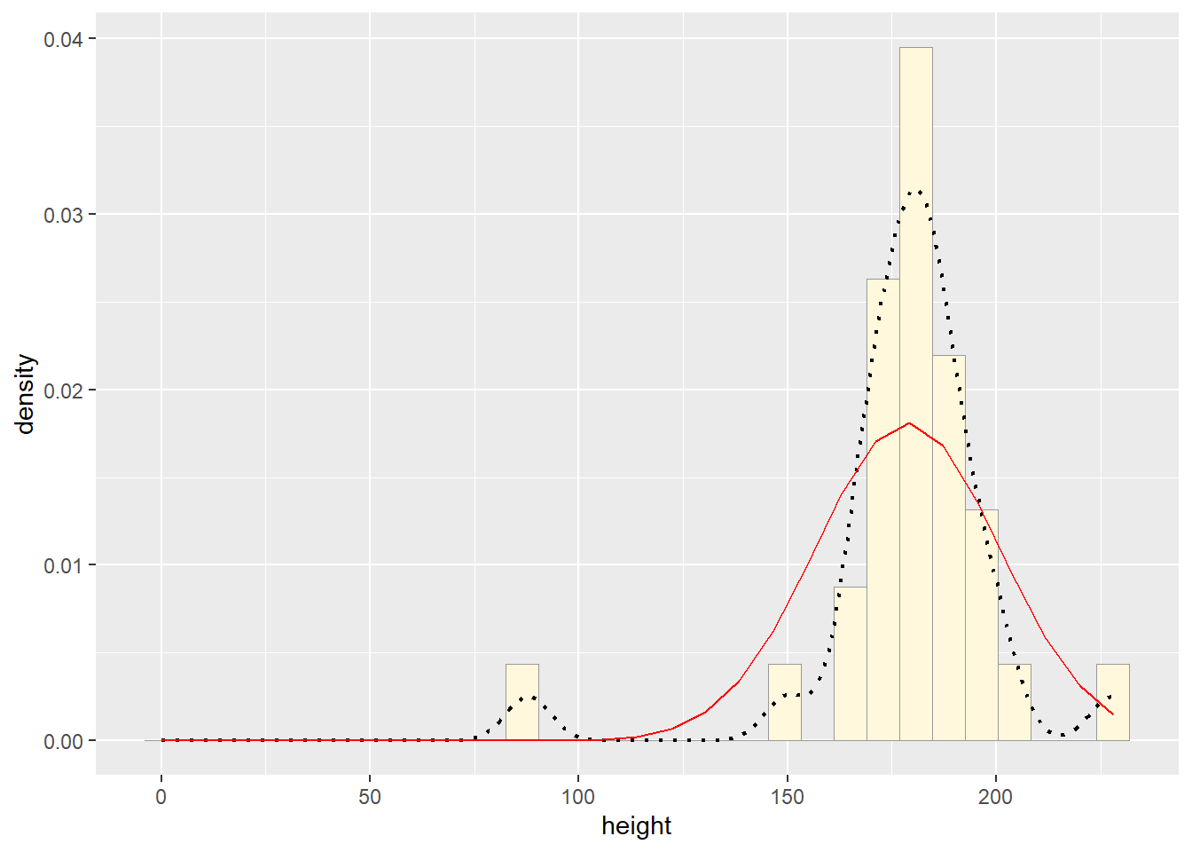
# plot exponential probability density
expoPars <- fitdistr(z$height,"exponential")
rateML <- expoPars$estimate["rate"]
stat2 <- stat_function(aes(x = xval, y = ..y..), fun = dexp, colour="blue", n = length(z$height), args = list(rate=rateML))
p1 + stat + stat2## `stat_bin()` using `bins = 30`. Pick better value with `binwidth`.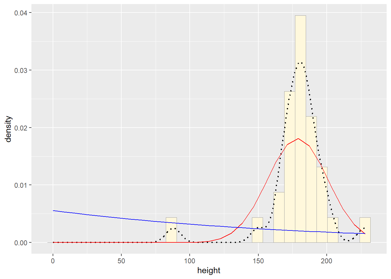
# plot uniform probability density
stat3 <- stat_function(aes(x = xval, y = ..y..), fun = dunif, colour="darkgreen", n = length(z$height), args = list(min=min(z$height), max=max(z$height)))
p1 + stat + stat2 + stat3## `stat_bin()` using `bins = 30`. Pick better value with `binwidth`.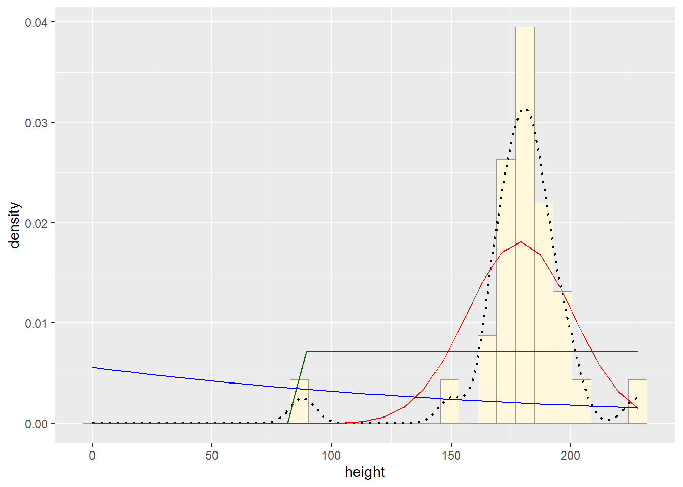
# plot gamma probability density
gammaPars <- fitdistr(z$height,"gamma")## Warning in densfun(x, parm[1], parm[2], ...): NaNs producedshapeML <- gammaPars$estimate["shape"]
rateML <- gammaPars$estimate["rate"]
stat4 <- stat_function(aes(x = xval, y = ..y..), fun = dgamma, colour="brown", n = length(z$height), args = list(shape=shapeML, rate=rateML))
p1 + stat + stat2 + stat3 + stat4## `stat_bin()` using `bins = 30`. Pick better value with `binwidth`.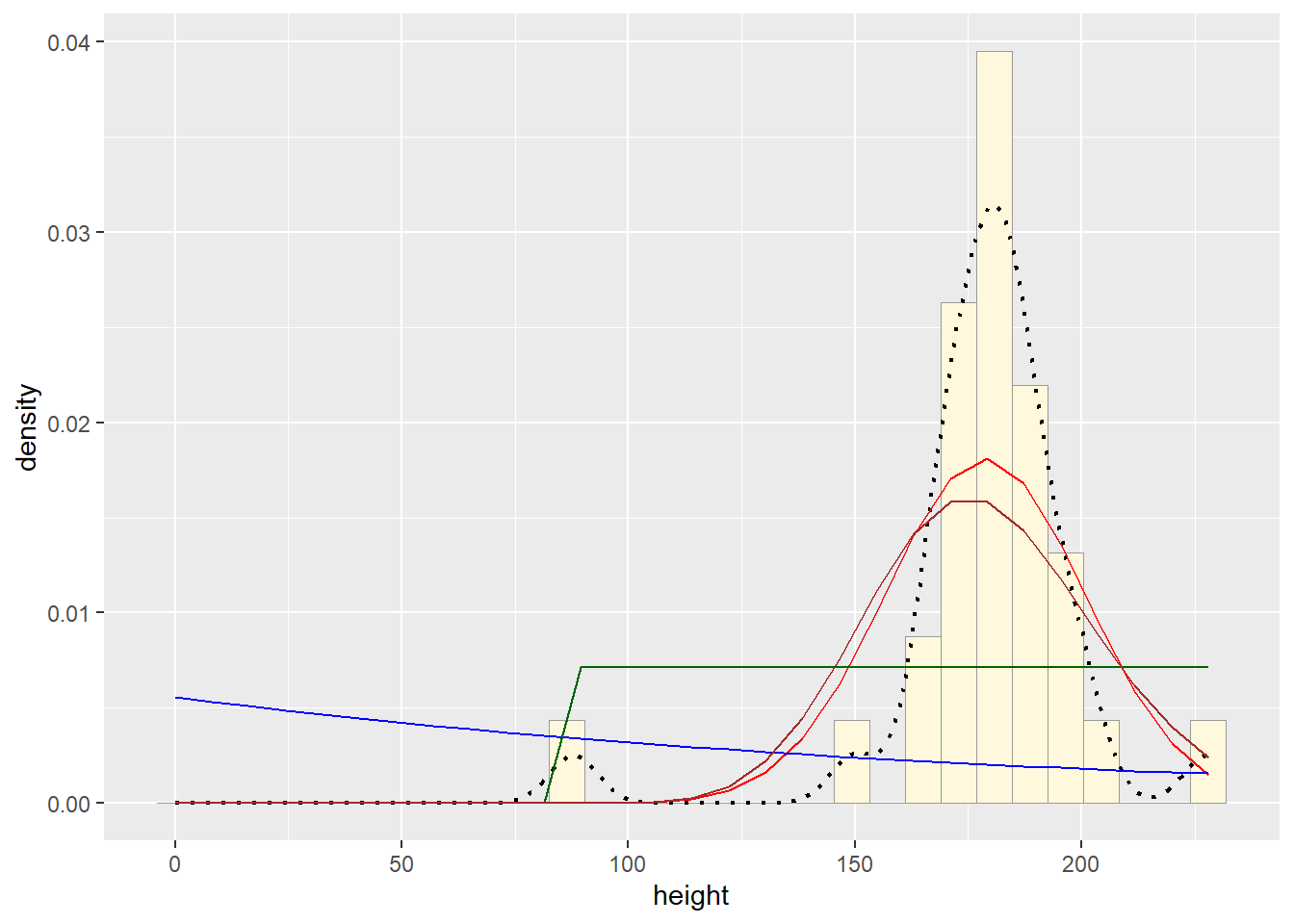
# plot beta probability density
pSpecial <- ggplot(data=z, aes(x=height/(max(height + 0.1)), y=..density..)) +
geom_histogram(color="grey60",fill="cornsilk",size=0.2) +
xlim(c(0,1)) +
geom_density(size=0.75,linetype="dotted")
betaPars <- fitdistr(x=z$height/max(z$height + 0.1),start=list(shape1=1,shape2=2),"beta")## Warning in densfun(x, parm[1], parm[2], ...): NaNs produced
## Warning in densfun(x, parm[1], parm[2], ...): NaNs producedshape1ML <- betaPars$estimate["shape1"]
shape2ML <- betaPars$estimate["shape2"]
statSpecial <- stat_function(aes(x = xval, y = ..y..), fun = dbeta, colour="orchid", n = length(z$height), args = list(shape1=shape1ML,shape2=shape2ML))
pSpecial + statSpecial ## `stat_bin()` using `bins = 30`. Pick better value with `binwidth`.## Warning: Removed 2 rows containing missing values or values outside the scale range
## (`geom_bar()`).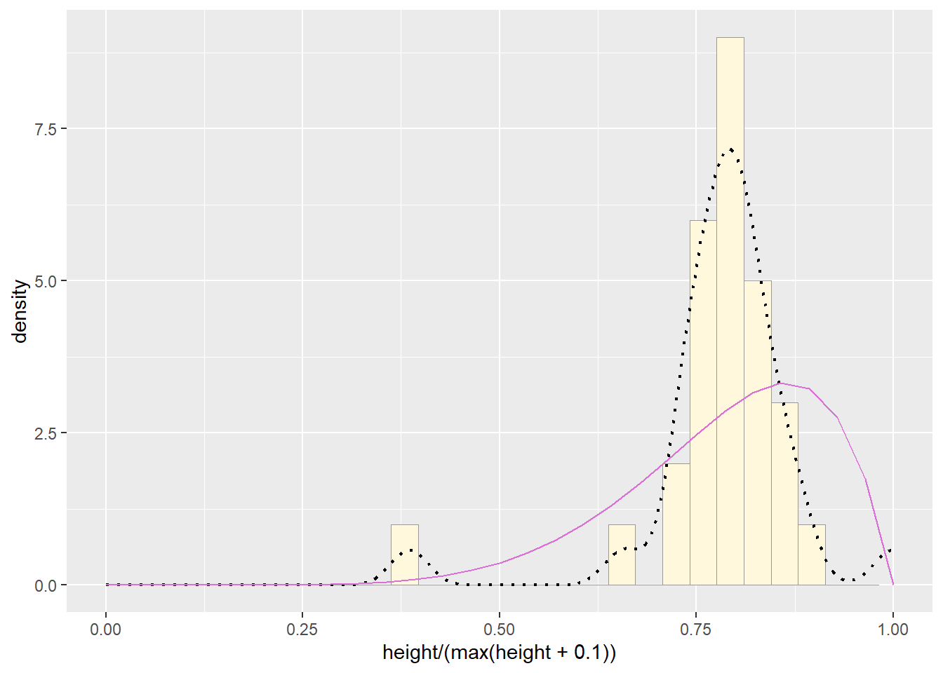
Question 3
Find the best-fitting distribution for your data.
The normal probability density curve was best fitting for the Starwars data we used. The beta curve actually fit most closely, but the normal probability density curve is more realistic than using something like a beta or uniform distribution, as these fix the upper bounds.Question 4
Simulate a new data set. Using the best-fitting distribution, go back to the code and get the maximum likelihood parameters. Use those to simulate a new data set, with the same length as your original vector, and plot that in a histogram and add the probability density curve. Right below that, generate a fresh histogram plot of the original data, and also include the probability density curve.## Simulated Plot ##
# read in data vector
d <- rnorm(n=29,mean=178.66)
d <- data.frame(1:29,d)
names(d) <- list("ID","height")
d <- d[d$height>0,]
str(d)## 'data.frame': 29 obs. of 2 variables:
## $ ID : int 1 2 3 4 5 6 7 8 9 10 ...
## $ height: num 177 179 179 178 181 ...summary(d$height)## Min. 1st Qu. Median Mean 3rd Qu. Max.
## 176.8 177.9 178.8 178.8 179.5 181.0# plot histogram of data
p1 <- ggplot(data=d, aes(x=height, y=..density..)) +
geom_histogram(color="grey60",fill="cornsilk", linewidth=0.2)
print(p1)## `stat_bin()` using `bins = 30`. Pick better value with `binwidth`.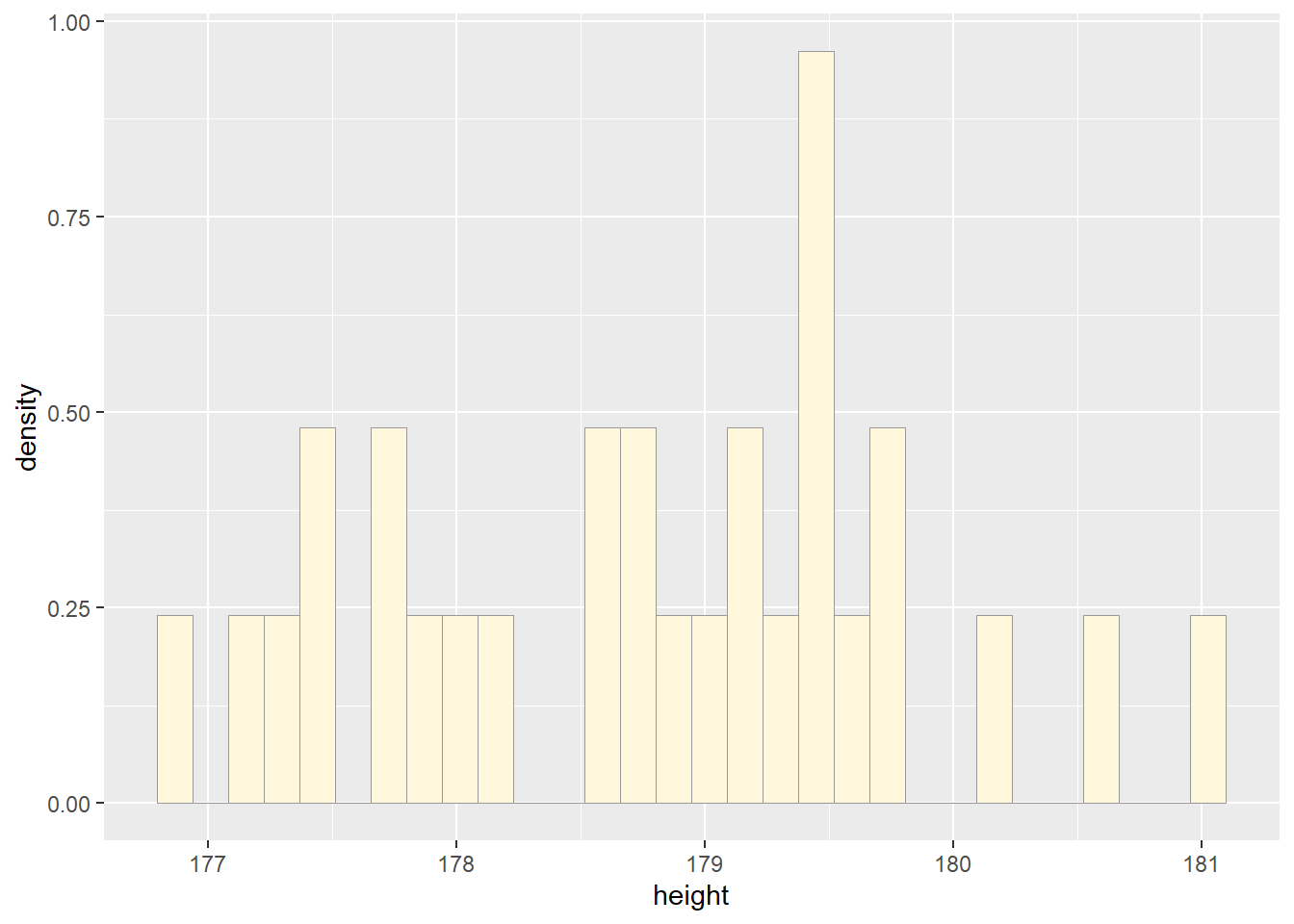
# add empirical density curve
p1 <- p1 + geom_density(linetype="dotted",size=0.75)
print(p1)## `stat_bin()` using `bins = 30`. Pick better value with `binwidth`.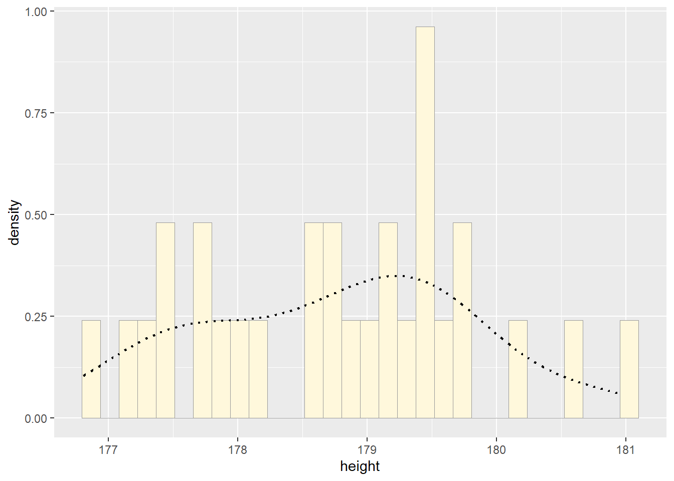
# get maximum likelihood parameters for normal
normPars <- fitdistr(d$height,"normal")
print(normPars)## mean sd
## 178.7727247 1.0352861
## ( 0.1922478) ( 0.1359397)str(normPars)## List of 5
## $ estimate: Named num [1:2] 178.77 1.04
## ..- attr(*, "names")= chr [1:2] "mean" "sd"
## $ sd : Named num [1:2] 0.192 0.136
## ..- attr(*, "names")= chr [1:2] "mean" "sd"
## $ vcov : num [1:2, 1:2] 0.037 0 0 0.0185
## ..- attr(*, "dimnames")=List of 2
## .. ..$ : chr [1:2] "mean" "sd"
## .. ..$ : chr [1:2] "mean" "sd"
## $ n : int 29
## $ loglik : num -42.2
## - attr(*, "class")= chr "fitdistr"normPars$estimate["mean"] # note structure of getting a named attribute## mean
## 178.7727### Original Plot ###
z0 <- data.frame(starwars)
z <- na.omit(starwars)
view(z)

# plot histogram of data
p1 <- ggplot(data=z, aes(x=height, y=..density..)) +
  geom_histogram(color="grey60",fill="cornsilk", linewidth=0.2)
print(p1)
## `stat_bin()` using `bins = 30`. Pick better value with `binwidth`.
# add empirical density curve
p1 <-  p1 +  geom_density(linetype="dotted",size=0.75)
print(p1)
## `stat_bin()` using `bins = 30`. Pick better value with `binwidth`.
# plot normal probability density
meanML <- normPars$estimate["mean"]
sdML <- normPars$estimate["sd"]

xval <- seq(0,max(z$height),len=length(z$height))

 stat <- stat_function(aes(x = xval, y = ..y..), fun = dnorm, colour="red", n = length(z$height), args = list(mean = meanML, sd = sdML))
 p1 + stat
## `stat_bin()` using `bins = 30`. Pick better value with `binwidth`.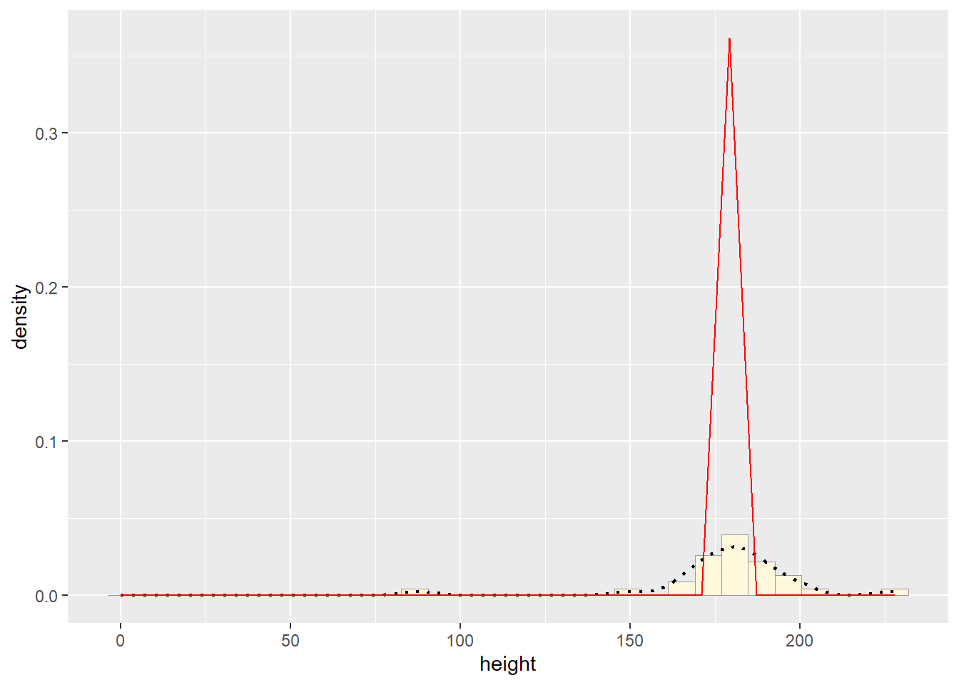
How do the two histogram profiles compare? Do you think the model is doing a good job of simulating realistic data that match your original measurements? Why or why not?
The two histograms are very different because we used the rnorm function which will create random data every time it’s run. We also have a very small data set (n=29) which makes it more difficult to notice variation.